This chapter uses the CSRD parks layer (csrd_parks.geojson). Click the file name to download it directly, then save it in your data/ folder. Source: Columbia Shuswap Regional District Open Data (ArcGIS Hub), Park Locations — 66 point features, WGS 84 (EPSG:4326).
Chapter goals
By the end of this chapter you will be able to:
Distinguish vector spatial data (points, lines, polygons) from raster spatial data (grids), and explain where each fits in a forestry workflow.
Explain the role of a CRS (coordinate reference system) and recognize three common ones: WGS84 (EPSG:4326), BC Albers (EPSG:3005), and Web Mercator (EPSG:3857).
Build an sf point object from a tibble of latitude and longitude using st_as_sf().
Read and write spatial files with st_read() and st_write() for shapefiles, GeoJSON, and GeoPackage formats.
Reproject between CRSs with st_transform().
Compute basic spatial operations: st_distance(), st_buffer(), st_intersection(), and st_area().
Plot spatial data inline in a Quarto report with geom_sf() (a ggplot2 geom).
Recognize that sf objects are tibbles with a special geometry column — every dplyr verb still works.
Expected output for this chapter
TipWhat you will hand in
A rendered Quarto HTML report (frst232_ch10_learner.html) containing:
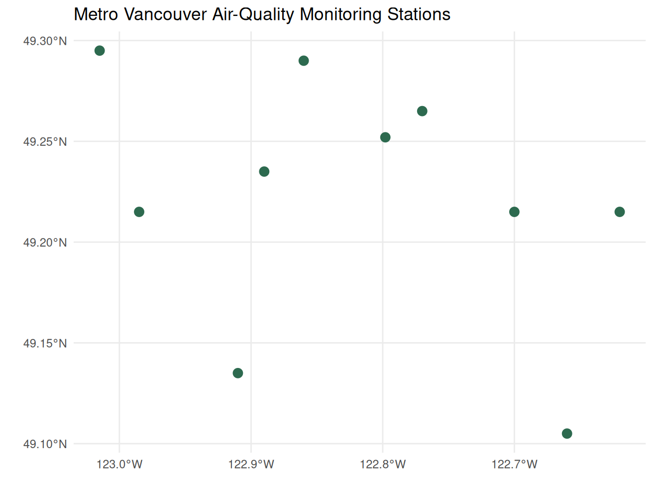
The Metro Vancouver air-quality stations as an sf point object built from the lat/lon tibble provided in this chapter.
A simple geom_sf() plot of the stations.
The pairwise distance matrix (in metres) between every pair of stations.
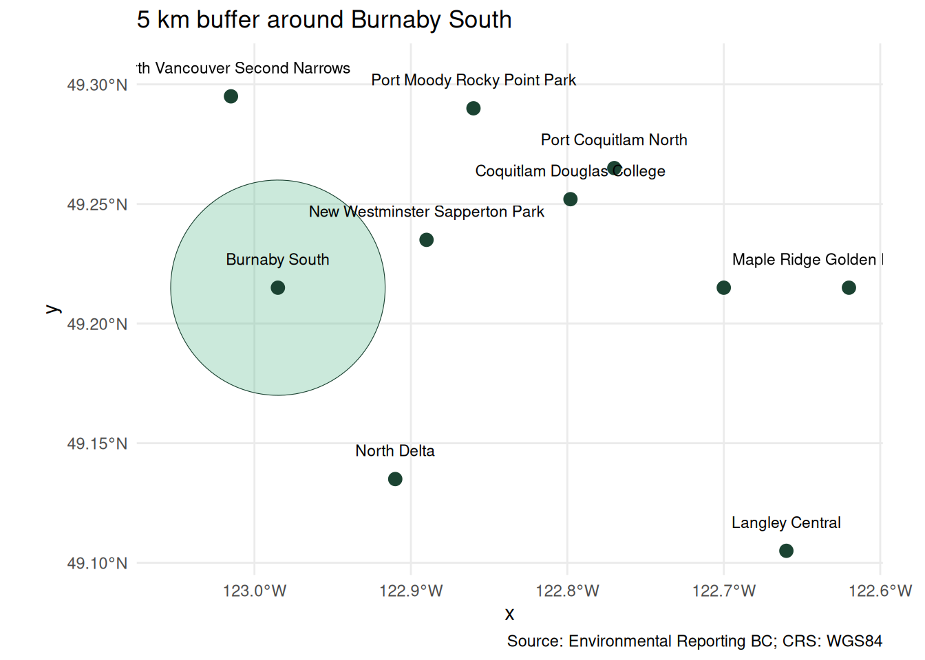
A 5 km buffer drawn around any one station, with both the original point and the buffer polygon plotted on the same chart.
One example of a CRS transformation (e.g., from WGS84 to BC Albers) with a one-sentence note on why you would reproject.
The corresponding .qmd source file.
A short group-lab worksheet (or screenshot) submitted to the course site.
2 Where we are
Through Chapter 9 you turned tibbles into charts. Chapter 10 turns tibbles into maps. The same air-quality stations you have been working with all term — Burnaby South, Coquitlam, Langley Central, etc. — are not just rows in a tibble. They are points in space with latitudes and longitudes. Once R knows that, you can:
Compute distances between them.
Buffer them by a radius.
Intersect them with watersheds, forest-district polygons, or fire perimeters.
Plot them on a map alongside any other spatial layer.
This is what “spatial data analysis” means in practice.
3 Installing sf
The sf package depends on three system libraries: GDAL, GEOS, and PROJ. On Posit Cloud, Windows, and Mac these are bundled — install.packages("sf") just works. On a fresh Linux install you may need to install the system libraries separately (sudo apt install libgdal-dev libgeos-dev libproj-dev).
install.packages("sf")library(sf)
If you cannot get sf to install locally, switch to Posit Cloud for this chapter. The cloud environment has everything pre-installed.
4 What is an sf object?
An sf object is a tibble with one extra column called geometry, plus a CRS attached. Every regular dplyr verb (filter, select, mutate, summarise, joins) still works on it. The geometry column is sticky — most operations preserve it automatically.
That single design decision — “spatial data is just a tibble” — is why sf integrates so cleanly with the rest of the tidyverse.
DEM (elevation), forest cover, fire scars from satellite
This chapter covers vector spatial data only. Raster in R (terra package) is a sequel topic, not required for FRST 232.
6 Coordinate Reference Systems (CRS) — the most-skipped step
Every spatial dataset has a CRS — the coordinate system its geometries are expressed in. Common ones for BC forestry work:
CRS
EPSG code
Units
Where used
WGS84 (latitude / longitude)
4326
degrees
GPS, web data, GeoJSON from internet
BC Albers Equal Area
3005
metres
BC Government data, all distance/area calculations in BC
Web Mercator
3857
metres
Online maps (Google Maps, Leaflet basemaps)
NAD83 / UTM Zone 10N
26910
metres
Field GPS in southern BC
Two rules:
A CRS is meaningless without units. Lat/lon is in degrees; BC Albers is in metres. Asking “what is the distance between these two points?” requires a metric CRS.
Two layers must share a CRS to be combined. If your stations are in WGS84 and a forest-district polygon is in BC Albers, you must reproject one of them first.
st_transform(data, crs = 3005) reprojects to a target CRS. Always check st_crs(data) after loading any new file.
7 Build an sf object from a tibble
The most common starting point: you have a tibble with latitude and longitude columns (e.g., GPS-collected field plots, station locations). Convert it to sf with st_as_sf():
# Approximate Metro Vancouver air-quality station coordinatesstations <-tribble(~location, ~lon, ~lat,"Burnaby South", -122.985, 49.215,"Coquitlam Douglas College", -122.798, 49.252,"Langley Central", -122.660, 49.105,"Maple Ridge Golden Ears School", -122.620, 49.215,"New Westminster Sapperton Park", -122.890, 49.235,"North Delta", -122.910, 49.135,"North Vancouver Second Narrows", -123.015, 49.295,"Pitt Meadows Airport", -122.700, 49.215,"Port Coquitlam North", -122.770, 49.265,"Port Moody Rocky Point Park", -122.860, 49.290)stations_sf <- stations |>st_as_sf(coords =c("lon", "lat"), crs =4326)stations_sf
Simple feature collection with 10 features and 1 field
Geometry type: POINT
Dimension:     XY
Bounding box:  xmin: -123.015 ymin: 49.105 xmax: -122.62 ymax: 49.295
Geodetic CRS:  WGS 84
# A tibble: 10 × 2
   location                                geometry
 * <chr>                                <POINT [°]>
 1 Burnaby South                  (-122.985 49.215)
 2 Coquitlam Douglas College      (-122.798 49.252)
 3 Langley Central                 (-122.66 49.105)
 4 Maple Ridge Golden Ears School  (-122.62 49.215)
 5 New Westminster Sapperton Park  (-122.89 49.235)
 6 North Delta                     (-122.91 49.135)
 7 North Vancouver Second Narrows (-123.015 49.295)
 8 Pitt Meadows Airport             (-122.7 49.215)
 9 Port Coquitlam North            (-122.77 49.265)
10 Port Moody Rocky Point Park      (-122.86 49.29)
What changed:
The lon and lat columns disappeared.
A new column geometry appeared, holding the point for each row.
A Geometry type:, Dimension:, Bounding box:, and Geodetic CRS: header now appears on print.
The tibble still has 10 rows; you can still call filter(), select(), mutate(), summarise(), and the joins on it.
Tipcoords = c("lon", "lat") — order matters
The first element is the x axis (longitude), the second is y (latitude). Many beginners write c("lat", "lon") — common bug, easy to spot (your points end up off the coast of Somalia, where lat 49 swapped with lon −122 plots).
8 Reproject — from WGS84 to BC Albers
For any distance or area calculation in BC, reproject to BC Albers (EPSG:3005), which has units in metres:
stations_bcalbers <- stations_sf |>st_transform(crs =3005)st_crs(stations_bcalbers)$Name # human-readable name
[1] "NAD83 / BC Albers"
st_bbox(stations_bcalbers) # bounding box in metres
# A tibble: 5 × 4
  from                           to                       distance_m distance_km
  <chr>                          <chr>                           [m]       <dbl>
1 Langley Central                North Vancouver Second …     33411.        33.4
2 North Vancouver Second Narrows Langley Central              33411.        33.4
3 Maple Ridge Golden Ears School North Vancouver Second …     30123.        30.1
4 North Vancouver Second Narrows Maple Ridge Golden Ears…     30123.        30.1
5 Burnaby South                  Langley Central              26692.        26.7
The pair with the longest distance is typically North Vancouver Second Narrows to Langley Central — opposite corners of Metro Vancouver.
10st_buffer() — circles around points
st_buffer(data, dist) returns a polygon for each input geometry, expanded by dist units. In a metric CRS, dist is in metres.
Simple feature collection with 1 feature and 1 field
Geometry type: POLYGON
Dimension:     XY
Bounding box:  xmin: 1214813 ymin: 466198.9 xmax: 1224813 ymax: 476198.9
Projected CRS: NAD83 / BC Albers
# A tibble: 1 × 2
  location                                                              geometry
* <chr>                                                            <POLYGON [m]>
1 Burnaby South ((1224813 471198.9, 1224806 470937.2, 1224785 470676.3, 1224751…
Practical use: “which forest stands are within 5 km of a proposed road?” Buffer the road by 5 km, then intersect with the stand polygons. That is a one-line spatial-overlay analysis.
11st_intersection() — overlay two layers
st_intersection(a, b) returns the geometric overlap of two spatial datasets. Useful for “which stations are inside this buffer?” and similar overlay questions:
# In hectares (1 ha = 10,000 m²)as.numeric(buffer_area_m2) /10000
[1] 7850.393
A 5 km buffer is a circle of radius 5,000 m, so area = π × 5000² ≈ 78.5 million m² ≈ 7,854 ha. The numbers should match (within rounding for the BC Albers projection).
13 Reading and writing files
13.1 Reading
# Shapefile (the .shp is the main file; .shx, .dbf, .prj must be alongside)districts <-st_read(here("data", "forest_districts.shp"))# GeoJSONparks <-st_read(here("data", "parks.geojson"))# GeoPackage (modern, single-file format — preferred)fire <-st_read(here("data", "fire_perimeters.gpkg"))
st_read() automatically detects the format from the extension and applies the CRS recorded in the file’s metadata. After every read, always check st_crs(data) to confirm what you got.
Recommendation: prefer GeoPackage (.gpkg) for new files. Shapefiles have a 10-character column-name limit, no field-name spaces, and split a single dataset across four files — all annoyances that GeoPackage fixes.
14 Plotting with geom_sf()
geom_sf() is a ggplot2 geom that draws sf geometries. It works the same as any other geom — no new grammar to learn:
Warning in st_point_on_surface.sfc(sf::st_zm(x)): st_point_on_surface may not
give correct results for longitude/latitude data
Notice: the buffer was computed in BC Albers (metric), then reprojected back to WGS84 for plotting alongside the lat/lon stations. Always reproject before combining layers.
15 A real spatial file: the CSRD parks layer
Everything so far used a small synthetic tibble. Now we read a real open-data file: the park point locations published by the Columbia Shuswap Regional District (CSRD). It is a single GeoJSON file — no shapefile bundle, no repository clone. (The download is scripted in scripts/download_csrd_parks.R.)
parks <-st_read(here("data", "csrd_parks.geojson"), quiet =TRUE)# Always inspect after readingnrow(parks) # how many features?
[1] 66
st_geometry_type(parks)[1] # points, lines, or polygons?
[1] POINT
18 Levels: GEOMETRY POINT LINESTRING POLYGON MULTIPOINT ... TRIANGLE
st_crs(parks)$input # which CRS did the file declare?
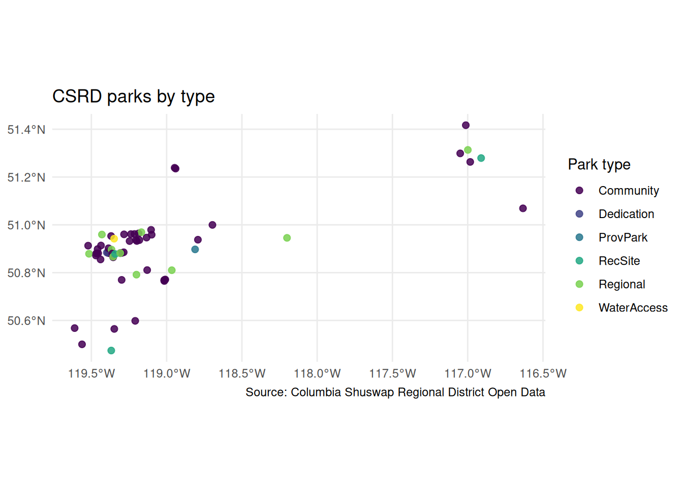
Now a static thematic map, coloured by park type, using the geom_sf() grammar from above:
ggplot(parks) +geom_sf(aes(colour = ParkType), size =2, alpha =0.85) +scale_colour_viridis_d() +labs(title ="CSRD parks by type",colour ="Park type",caption ="Source: Columbia Shuswap Regional District Open Data") +theme_minimal()
This is the static counterpart to the interactive leaflet map you will build in Chapter 11 — the same data, the same question, two presentation choices.
For a working forestry analyst, this catalogue is the most important single bookmark in BC. Most layers are published under the Open Government Licence — British Columbia, but some carry other terms (a few are restricted or personal-use only), so check each dataset’s licence before you redistribute. Formats vary too: many layers offer a shapefile or GeoJSON, while others come as CSV, KML, or a live ArcGIS/WMS service — pick the format your workflow needs.
To use one of these in your project:
Download from the catalogue.
Unzip into data/ inside your frst232/ project.
Read with st_read(here("data", "filename.shp")).
Check st_crs(data) and reproject to BC Albers if needed.
Plot with geom_sf() or combine with other layers using st_intersection().
17 Spatial joins — st_join()
When you have two layers and want to attach attributes of one to the other based on spatial position, use st_join():
# Suppose `districts_sf` is a polygon layer of forest districts.# Add the district name to each station based on which district it falls in:stations_with_district <-st_join(stations_sf, districts_sf, join = st_within)
st_within means “join station to district where the station is inside the district”. Other join predicates: st_intersects, st_touches, st_overlaps, st_nearest_feature.
A spatial join is the GIS equivalent of left_join() from Chapter 6 — except the key is geometric position, not a shared column.
Simple feature collection with 3 features and 1 field
Geometry type: POINT
Dimension:     XY
Bounding box:  xmin: -122.86 ymin: 49.215 xmax: -122.7 ymax: 49.29
Geodetic CRS:  WGS 84
# A tibble: 3 × 2
  location                            geometry
* <chr>                            <POINT [°]>
1 Pitt Meadows Airport         (-122.7 49.215)
2 Port Coquitlam North        (-122.77 49.265)
3 Port Moody Rocky Point Park  (-122.86 49.29)
# select — works (geometry stays sticky)stations_sf |>select(location)
Simple feature collection with 10 features and 1 field
Geometry type: POINT
Dimension:     XY
Bounding box:  xmin: -123.015 ymin: 49.105 xmax: -122.62 ymax: 49.295
Geodetic CRS:  WGS 84
# A tibble: 10 × 2
   location                                geometry
   <chr>                                <POINT [°]>
 1 Burnaby South                  (-122.985 49.215)
 2 Coquitlam Douglas College      (-122.798 49.252)
 3 Langley Central                 (-122.66 49.105)
 4 Maple Ridge Golden Ears School  (-122.62 49.215)
 5 New Westminster Sapperton Park  (-122.89 49.235)
 6 North Delta                     (-122.91 49.135)
 7 North Vancouver Second Narrows (-123.015 49.295)
 8 Pitt Meadows Airport             (-122.7 49.215)
 9 Port Coquitlam North            (-122.77 49.265)
10 Port Moody Rocky Point Park      (-122.86 49.29)
# summarise — also works (returns a multi-point or aggregated geometry)stations_sf |>mutate(group =if_else(str_detect(location, "Vancouver"), "Vancouver", "Other")) |>group_by(group) |>summarise(n =n(), .groups ="drop")
Simple feature collection with 2 features and 2 fields
Geometry type: GEOMETRY
Dimension:     XY
Bounding box:  xmin: -123.015 ymin: 49.105 xmax: -122.62 ymax: 49.295
Geodetic CRS:  WGS 84
# A tibble: 2 × 3
  group         n                                                       geometry
  <chr>     <int>                                                 <GEOMETRY [°]>
1 Other         9 MULTIPOINT ((-122.66 49.105), (-122.62 49.215), (-122.7 49.21…
2 Vancouver     1                                        POINT (-123.015 49.295)
The geometry column comes along for the ride. This is the single biggest reason sf works so well: nothing new to learn beyond the spatial operations themselves.
19 Active learning
19.1 Activity 1 — Build the sf object
Build stations_sf from the stations tibble. Confirm nrow(stations_sf) is 10 and st_crs(stations_sf)$Name says "WGS 84".
19.2 Activity 2 — Reproject
Reproject stations_sf to BC Albers (EPSG:3005). What units does st_bbox() now report?
19.3 Activity 3 — Distances
Compute the pairwise distance matrix in metres. What is the distance (in km) from Burnaby South to Langley Central?
19.4 Activity 4 — Buffer
Build a 10 km buffer around North Vancouver Second Narrows. Which stations fall inside it? Use st_intersection() to find out.
19.5 Activity 5 — Plot
Plot all the stations with geom_sf() and add a title. Save the plot as a 7×5 inch PNG.
20 Group lab activity
NoteLab: Build a station map together
Work in groups of 3 or 4. Each member starts from the same stations tibble.
Task 1 — Build the sf object. Each member runs st_as_sf() to build stations_sf. Confirm everyone gets the same result.
Task 2 — Pick a buffer radius. Discuss: for a smoke-exposure analysis, what radius makes sense around each station? (Often 5 km for community exposure, larger for regional estimates.) Pick a number.
Task 3 — Buffer all stations. Apply st_buffer() to all 10 stations at the chosen radius.
Task 4 — Find overlapping pairs. Use st_intersects() to find pairs of stations whose buffers overlap. Hint: st_intersects(buffers_sf, buffers_sf) returns a list of indices.
Task 5 — Plot it. Build a single geom_sf() plot showing all the buffer polygons (with fill mapped to a colour) and all the station points on top.
Task 6 — Caption. Write a one-sentence caption explaining what the chart shows.
Task 7 — Submit. Submit the rendered chart, the buffer radius chosen, the code, and the caption.
21 Exercises
Build sf. Build stations_sf from the stations tibble. Confirm with class(stations_sf) that the result is an sf object.
Reproject. Reproject stations_sf to BC Albers (EPSG:3005). Compare st_bbox() of both — what are the units of each?
Pairwise distances. Compute and print the pairwise distance matrix in kilometres. What is the longest distance? Between which two stations?
Buffer + intersection. Build a 7.5 km buffer around Burnaby South. Use st_intersection() to find which other stations fall inside it. Report the list of station names.
geom_sf plot. Plot all stations with geom_sf(), then add labels with geom_sf_text(aes(label = location), size = 3). Save as a PNG.
Write a GeoJSON. Save stations_sf to outputs/stations.geojson with st_write(). Open the resulting file in a text editor — what does the JSON structure look like?
Area of a buffer. Compute the area in hectares of the 5 km buffer around any station. Confirm it is approximately π × 5000² / 10,000 ≈ 7,854 ha.
Optional, harder. Download the BC provincial boundary from the BC Data Catalogue. Load it with st_read(). Plot it as a polygon with geom_sf(), then overlay your stations on top.
Common spatial mistakes — spot the bug. For each case, say what is wrong and how to fix it:
st_distance() is run on a lon/lat (EPSG:4326) object and the result is read as metres.
An sf object is built with st_as_sf(coords = c("lat", "lon")) (axes reversed), so the points land in the wrong place.
A 5 km buffer is built before reprojecting from lon/lat to a metric CRS, so dist = 5000 is treated as 5000 degrees.
22 Optional, advanced
22.1 Spatial joins
A spatial join attaches attributes of one layer to another based on geometric predicates. Most common predicates:
st_within() — point inside polygon
st_intersects() — any geometric overlap
st_touches() — share a boundary but do not overlap
st_nearest_feature() — nearest neighbour
st_join(points, polygons, join = st_within)
22.2 Caching downloaded files
After you st_read() a downloaded shapefile, save it locally as a GeoPackage:
Subsequent reads from .gpkg are faster and avoid the shapefile’s quirks.
22.3 Validating geometries
Sometimes a downloaded polygon layer has invalid geometries (self-intersections, slivers). Use:
districts_valid <- districts |>st_make_valid()
before any overlay operations.
23 A glimpse of Chapter 11: From static maps to interactive maps
In Chapter 11 you take the same stations_sf object and put it on an interactive web map using the leaflet package. Pan, zoom, click for popups — the difference between a static PNG and a slippy map is the difference between a report and a tool.
Static (Ch 10, geom_sf)
Interactive (Ch 11, leaflet)
Fixed extent
Pan + zoom
No popups
Click a point for info
Print-friendly
Web-deliverable
One basemap
Many basemap choices (street, satellite, terrain)
The two are complementary. Static maps for reports; interactive maps for dashboards and field handoff.
24 Self-assessment quiz
1. The two main paradigms for representing spatial data are —
2D and 3D
vector (points, lines, polygons) and raster (grid of cells)
SVG and PDF
XML and JSON
Vector for discrete shapes; raster for continuous fields like elevation or satellite imagery.
2. An sf object in R is —
A completely new data structure unrelated to tibbles
A tibble with one extra column called geometry, plus a CRS
A shapefile
A list of coordinates
That tibble-like design is why every dplyr verb still works on an sf object.
3. The CRS code for WGS84 (latitude / longitude) is —
3005
4326
3857
26910
EPSG:4326 = WGS84. EPSG:3005 = BC Albers. EPSG:3857 = Web Mercator.
4. The CRS code for BC Albers (the standard for BC Government data) is —
4326
3005
3857
26910
EPSG:3005 — equal-area projection used for nearly all BC forestry spatial data. Units are metres.
5. You have point data in lat/lon (degrees). To compute the distance between two points in metres, you must —
Use Pythagoras on the degrees
Reproject to a metric CRS (e.g., BC Albers, EPSG:3005), then use st_distance()
Convert degrees to metres manually with 111000
Use raster algebra
Distance in degrees is meaningless because degrees of longitude vary with latitude. Reproject to a metric CRS first.
6. st_as_sf(coords = c("lon", "lat"), crs = 4326) tells R that —
lon is y and lat is x
lon (x) and lat (y) columns in the tibble define point geometries in WGS84
The data should be plotted but not stored
The data is in BC Albers
Order matters: first is x (longitude), second is y (latitude). Swapping them is a common bug.
7. st_transform(data, crs = 3005) does what?
Adds an attribute column
Reprojects the data to BC Albers, transforming the coordinates so they are still in the right place but in metres
Deletes the geometry
Plots the data
Reprojection is mathematical — the geometries move from one coordinate system to another while keeping the real-world position.
8. st_buffer(point, dist = 5000) in a CRS with metres returns —
A point 5,000 metres away
A polygon representing a circle of radius 5,000 metres around the point
A line of length 5,000 m
An error
In a metric CRS, dist is in metres. So 5000 = 5 km buffer.
9. st_intersection(layer_a, layer_b) returns —
The union of both layers
The geometric overlap of the two layers
Only the attributes of layer_b
An error
Intersection is the geometric AND — the area, line, or points where both layers overlap.
10. geom_sf() is —
A completely separate plotting system from ggplot2
A ggplot2 geom that draws sf geometries (points, lines, polygons) using ggplot's grammar
A function in the leaflet package
A way to save sf objects
geom_sf() uses the same ggplot grammar as every other geom — same +, same labs(), same themes.
11. To read a shapefile in R, you use —
read_csv()
st_read()
read_excel()
readRDS()
st_read() reads any vector spatial format and auto-detects from the extension.
12. The recommended new-data file format (over shapefile) is —
CSV with WKT
GeoPackage (.gpkg) — single file, no column-name limits
Excel
Plain text
GeoPackage is a modern single-file format that fixes shapefile's limitations (10-char column names, no spaces, 4 separate files per layer).
13. A spatial join (st_join) is the GIS equivalent of —
filter()
left_join() — but matched on geometric position instead of a shared column
summarise()
pivot_wider()
Where left_join matches on a shared key column, st_join matches on geometric predicates like "within" or "intersects".
14. You loaded a new spatial file. What is the first command you should run?
plot(data)
summary(data)
st_crs(data) to confirm the coordinate reference system
nrow(data)
Without knowing the CRS, you cannot safely combine, transform, or compute distances. Always check the CRS first.
15. st_area() on a polygon in BC Albers returns area in —
degrees squared
square metres
hectares
acres
BC Albers' units are metres, so areas come out in m². To convert to hectares, divide by 10,000.
16. dplyr verbs on an sf object —
Strip the geometry column
Keep the geometry column automatically (it is "sticky")
Do not work — you need separate spatial verbs
Convert the data to a base R data.frame
The geometry column survives filter, select, mutate, summarise, and joins. To drop it explicitly, use st_drop_geometry().
17. When you have two sf layers and want to combine them on a plot, you must first —
Convert both to data.frames
Make sure they share a CRS (or reproject one to match the other)
Save both to disk
Pivot one of them longer
Plotting or any geometric operation on two mismatched-CRS layers either errors or gives nonsense. Reproject first.
18. For BC forestry spatial data, the canonical source is —
A textbook
The BC Data Catalogue (https://catalogue.data.gov.bc.ca/) — Open Government Licence BC
Wikipedia
A private consulting firm
Forest districts, cut blocks, fire perimeters, watersheds, ownership — all openly published.
19. The single most common bug when building an sf object from a lat/lon tibble is —
Forgetting to load tidyverse
Passing coords = c("lat", "lon") instead of c("lon", "lat") — first is x, second is y
Using too many decimal places
The wrong package version
Swapping lat and lon plots your BC points off the coast of Somalia. Look at the bounding box to spot it.
20. Reflection. Until now your forestry analysis treated rows as anonymous records. How does adding spatial location change what questions you can answer?
Common reflections: I can now ask "how close" instead of just "how many" · buffers let me reason about exposure zones, fire risk, road influence · intersection lets me cross datasets that share nothing but location · plotting on a map immediately surfaces patterns that a table hides · the biggest unlock is that BC Data Catalogue is now usable from R — every shapefile becomes a line of code instead of a manual import.
25 AI as a debugging companion
TipUseful prompts
“My ggplot of an sf object plots the points off the coast of Africa. What did I do wrong?” (Answer: swapped lat and lon in coords = c(...).)
“How do I find which of my stations are inside this polygon?” (Answer: st_join(stations, polygon, join = st_within) or st_intersection(stations, polygon).)
“My st_distance() returns numbers in millions. What units are those in?” (Answer: the units of the current CRS — for BC Albers, metres.)
26 Reading
Geocomputation with R (Lovelace, Nowosad, Muenchow) — the canonical free book on R spatial. Chapters 1–3 are required. https://r.geocompx.org/
The hardest concept this chapter is CRS. Spend a full lecture on it. Demo the “off the coast of Africa” bug live — show how degrees vs metres change everything.
The “sf objects are tibbles” message is the single biggest unlock. Once learners realise every dplyr verb still works, spatial work stops feeling like a different world.
Posit Cloud is strongly recommended for this chapter. Local sf installs sometimes fail on Linux and Mac without the right system libraries; cloud sidesteps all of it.
26.1 Materials provided
File
Purpose
frst232_ch10_learner.qmd
Quarto starter with TODO chunks.
frst232_ch10_solutions.qmd
Completed solutions. Do not distribute.
quiz_ch10.html
Standalone interactive quiz.
26.2 Reference numbers
Quantity
Approximate value
nrow(stations_sf)
10
st_crs(stations_sf)$Name
“WGS 84”
Burnaby South → Langley Central distance
~30 km
North Vancouver → Langley Central distance (longest pair)
~37 km
Area of 5 km buffer
~7,854 ha
26.3 Common stumbling points
Coords order.coords = c("lat", "lon") is the single most common bug. Insist on always checking with st_bbox() after building.
CRS confusion. Symptom: distances of “0.0003” (degrees) or “millions” (metres). Always check st_crs() and convert to a metric CRS before measuring.
Plotting two layers with mismatched CRSs. ggplot will often just plot the second layer in the first layer’s CRS, giving a wrong-looking map. Reproject explicitly.
Shapefile column-name surprises. A shapefile column named forest_district_name_long will arrive truncated to forst_dst_. Use GeoPackage going forward.