bc <- read_excel(here("data", "bc_disturbance_reforestation.xlsx"),
                 sheet = "Data")
dim(bc)
[1] 37 8The end-to-end case study uses the BC silviculture workbook (bc_disturbance_reforestation.xlsx). Click the file name to download it directly, then save it in your data/ folder. For the source and details, see the Datasets Used in This Book page.
By the end of this chapter you will be able to:
A complete end-to-end case-study report: take one of the course datasets, start from the raw file, document your cleaning, summarize by group, produce one figure (and an optional map only if you used the spatial extension), and render it as a single Quarto HTML report. This is both your final review and the best possible exam practice.
You started in Excel (Chapters 1–3), crossed the bridge into R (Chapter 4), and built — one chapter at a time — every stage of a reproducible analysis:
| Stage | You learned it in | Key functions |
|---|---|---|
| Import | Ch 4–5 | read_excel(), read_csv(), here() |
| Inspect | Ch 5 | glimpse(), summary(), dim(), colSums(is.na()) |
| Clean | Ch 6 | select(), filter(), rename(), mutate(), case_when() |
| Summarize | Ch 7 | group_by(), summarise(), count(), n_distinct() |
| Reshape | Ch 8 | pivot_longer(), pivot_wider() |
| Join | Ch 8 | left_join(), the filtering joins, pre/post-join checks |
| Visualize | Ch 9 | ggplot2, geoms, facets, themes, fig-alt |
| Render | Ch 5–12 | Quarto: code + prose + output in one document |
This chapter threads them all together.
We use one dataset — the BC silviculture file you have known since Chapter 1 — and run it through the whole pipeline.
bc <- read_excel(here("data", "bc_disturbance_reforestation.xlsx"),
sheet = "Data")
dim(bc)[1] 37 8glimpse(bc)Rows: 37
Columns: 8
$ Fiscal_Year <dbl> 1987, 1988, 1989, 1990, 1991, 1992, 1993…
$ Clearcutting_ha <dbl> 216304.92, 217836.07, 190635.52, 172360.…
$ Clearcutting_with_reserves_ha <dbl> 5800.400, 1842.952, 1456.666, 1400.013, …
$ Partial_cutting_ha <dbl> 20076.681, 31878.294, 23785.954, 18930.8…
$ Harvested_ha <dbl> 242182.0, 251557.3, 215878.1, 192691.6, …
$ Natural_Disturbance_ha <dbl> 20875.00, 9641.20, 10711.80, 28300.70, 1…
$ Total_Disturbance_ha <dbl> 263057.0, 261198.5, 226589.9, 220992.3, …
$ Reforestation_ha <dbl> 201972.5, 221296.3, 237275.9, 260370.8, …colSums(is.na(bc)) # missing values per column Fiscal_Year Clearcutting_ha
0 0
Clearcutting_with_reserves_ha Partial_cutting_ha
0 0
Harvested_ha Natural_Disturbance_ha
0 0
Total_Disturbance_ha Reforestation_ha
0 0 We add a decade grouping variable and a reforestation ratio (reforested area per hectare harvested), documenting each step as we go:
bc_clean <- bc |>
  mutate(
    decade          = (Fiscal_Year %/% 10) * 10,
    reforest_ratio  = Reforestation_ha / Harvested_ha
  )
bc_clean |> select(Fiscal_Year, decade, Harvested_ha,
                   Reforestation_ha, reforest_ratio) |> head()
# A tibble: 6 × 5
Fiscal_Year decade Harvested_ha Reforestation_ha reforest_ratio
<dbl> <dbl> <dbl> <dbl> <dbl>
1 1987 1980 242182 201972. 0.834
2 1988 1980 251557. 221296. 0.880
3 1989 1980 215878. 237276. 1.10
4 1990 1990 192692. 260371. 1.35
5 1991 1990 213217. 245370. 1.15
6 1992 1990 234086. 224983. 0.961by_decade <- bc_clean |>
group_by(decade) |>
summarise(
n_years = n(),
mean_harvest_ha = round(mean(Harvested_ha, na.rm = TRUE)),
mean_reforest_ha = round(mean(Reforestation_ha, na.rm = TRUE)),
mean_ratio = round(mean(reforest_ratio, na.rm = TRUE), 2),
.groups = "drop"
)
by_decade |> kable()| decade | n_years | mean_harvest_ha | mean_reforest_ha | mean_ratio |
|---|---|---|---|---|
| 1980 | 3 | 236539 | 220182 | 0.94 |
| 1990 | 10 | 203694 | 236134 | 1.17 |
| 2000 | 10 | 207063 | 221916 | 1.09 |
| 2010 | 10 | 204947 | 218683 | 1.08 |
| 2020 | 4 | 124579 | 209047 | 1.76 |
Note the discipline from Chapter 7: n_years is reported beside every mean, so a reader can see that the 1980s and 2020s decades are partial.
bc_long <- bc_clean |>
  select(Fiscal_Year, Harvested_ha, Reforestation_ha) |>
  pivot_longer(-Fiscal_Year, names_to = "series", values_to = "area_ha")

ggplot(bc_long, aes(Fiscal_Year, area_ha, colour = series, linetype = series)) +
  geom_line(linewidth = 1) +
  scale_colour_manual(values = c("#B7791F", "#2D6A4F"),
                      labels = c("Harvested", "Reforested")) +
  scale_linetype_manual(values = c("solid", "dashed"),
                        labels = c("Harvested", "Reforested")) +
  labs(title = "BC harvest and reforestation, 1987–2023",
       x = "Fiscal year", y = "Area (hectares)",
       colour = NULL, linetype = NULL,
       caption = "Source: Environmental Reporting BC") +
  theme_minimal()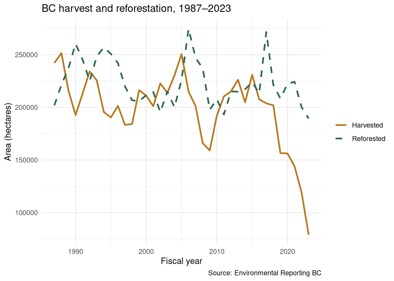
Everything above lives in one .qmd file. Pressing Render produces a single HTML report that another analyst can reproduce from the raw file — no hidden clicks, no copy-paste. That reproducibility is the whole point of this course.
The exam is not about memorizing function names — it is about recovering when something breaks. When you hit an error, climb this ladder one rung at a time:
object not found → object; could not find function → package not loaded; an unexpected number of rows → data.)glimpse(), summary(), dim(), names(). Most “code” bugs are really data surprises.When studying, AI is excellent for explaining an error or generating practice variants. Paste the exact error, your R and package versions, and the code you tried. Then verify the explanation against ?function_name and a small test — the same discipline the rest of the book taught. In a closed-book exam, the ladder above is what you carry in your head.
Run the seven-step pipeline above on a different course dataset (Ontario forest stats, or the cleaned air-quality file). Produce one summary table and one figure.
Introduce a deliberate bug (misspell a column, drop a library(), swap lat/lon). Use the debugging ladder to find and fix it. Write one sentence per rung.
Move your .qmd and data/ to a fresh folder and render. Does it work with no manual steps? If not, find the hidden dependency.
This course is a foundation. Natural next steps:
sf, raster data with terra, and remote sensing for forest inventory.renv, Git/GitHub, and parameterized Quarto reports for production work.Recommended reading mixes canonical and diverse voices:
Across the book’s chapters, AI has been a verification companion, not an author: it explains errors, drafts starting code, and suggests alternatives — and you check every line against the data and the documentation. That habit, more than any single function, is what makes you employable in a world where code is cheap and judgment is scarce.
sf is an optional extension and is not required on the exam.)library() calls; data paths that work locally but not from a clean project; reading NA as zero.Use AI as a verification and debugging partner, not an answer machine. The goal is not to make AI do the work — it is to use AI to help you understand, check, and improve your own work.
Fill in the brackets and paste this into your AI assistant. It should explain and check, not hand you a final assignment answer:
“I am working on FRST 232, this chapter. My dataset is
[file name]with columns[columns]. My task is[what you are trying to do]. I tried[paste your code or steps]and got[paste the exact output or error]. Explain what this does line by line, tell me whether it answers the question, and list the checks I should run to verify it. Do not give me the final answer.”
Verify it yourself — before trusting any result (yours or an AI’s):
filter() or a join;Common AI mistakes to watch for: inventing a column, function, or value that is not in your data; choosing a tool before reading the question; and (in Excel) suggesting the wrong cell range or forgetting to refresh a PivotTable.
When a reference solution is available, do not just copy it — use it to check your own work:
Write a prompt that would guide an AI toward the reference solution without handing over the final answer. Include the dataset, the columns, the task goal, the output format you need, and the verification checks. Then paste (or summarise) the AI’s response and answer: did its approach match the book’s? did it miss a verification step? did it invent a column, function, or value? what did your group change after checking it?